Implementing an Array Deque

A deque (pronounced as 'deck') is a double-ended queue: it allows a user to add and remove data from both ends. Another way of looking at deques is that they are concurrently stacks and queues, thus allowing them to combine the LIFO (last-in first-out) and FIFO (first-in first-out) functionalities.



Explicitly, an array deque has the capability of performing the following operations on each end:

1) Peek: You can look at the very first and last elements (entries of data) in the array-deque with a time-complexity of \(O(1)\).

2) Insert: You can insert ('push') an element to the back of the array deque with a time-complexity of \(O(1)\). To do this, the underlying algorithm just adds another element to the end of the array deque and updates the Tail to make it point to the last element in the deque. Somewhat similarly, you can insert an element to the front of the array deque with a time-complexity of \(O(n)\). To do this, the underlying algorithm just shifts all the elements in the array deque to the right by one position, and inserts the new element at the first entry.

3) Delete: You can delete ('pop') an element from the front and back of the array deque with a time complexity of \(O(1)\) by simply shifting the Head pointer by \(+1\) or the Tail pointer by \(-1\).

Implementing a Doubly Linked-List Deque

I then did my first layer of abstraction - converting the array-deque to a doubly linked-list deque. A doubly linked-list deque has the same functionalities as the array-deque, but is so much more efficient. Firstly, each data element is stored in a node. The node, in addition to containing the data, also contains a pointer to the node preceding it and the node following it, thus defining a natural ordering for the data contained in the structure. The two exceptions to this rule are the Head and Tail nodes which only have pointers to the start-point and end-point of the deque.



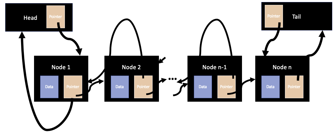
A doubly linked-list deque has the capability of performing the following operations on each end:

1) Peek: As before, you can look at the very first and last elements (entries of data) in the doubly linked-list deque with a time-complexity of \(O(1)\).

2) Insert: You can insert ('push') an element to the back of the doubly linked-list deque with a time-complexity of \(O(1)\) To do this, the underlying algorithm starts by creating a node that contains the new element. It then uses the Tail pointer node to access the 'last data-storing node' in the deque, and changes the pointers of both these nodes to point to the new node. It finally changes the pointers of the new node to point to the previous last node and the Tail pointer node, respectively. Similarly, you can insert an element to the front of the array deque with a time-complexity of \(O(1)\). To do this, the underlying algorithm similarly starts by creating a node that contains the new element. It then uses the Head pointer node to access the 'first data-storing node' in the deque, and changes the pointers of both these nodes to point to the new node. It finally changes the pointers of the new node to point to the Head pointer node and the previous first note, respectively. Thus, the new node is inserted into the data-structure.

3) Delete: You can delete ('pop') an element from the front and back of the doubly linked-list deque with a time complexity of \(O(1)\) by simply altering the pointers such that the Head (Tail) pointer points to the node after (before) 'the node to be deleted', so that the node in after (before) of the 'node to be deleted' instead points to the Head (Tail) pointer.

Implementing a Circular Array Fixed-Size Queue

I then wrote my second (and final) layer of abstraction - converting the doubly linked-list deque to the circular array fixed-size queue that I needed to implement the algorithm for the sound synthesizer. A circular array fixed-size queue uses the doubly linked-list functionality to perform the tasks of enqueuing at the Tail node and dequeuing at the Head node, while ensuring that there are atmost a fixed number of elements in the queue. The static size of the queue is not a constraint of the queue; rather, it is a feature: restricting the size of the queue can be done by storing its size and using a conditional statement to ensure that the capacity is not exceeded. Whenever an element in inserted to (deleted from) the queue, we move the tail index (head index) forward, while wrapping around the queue; so, the first (last) positional node is not necessarily the first (last) node in terms of the ordering of the data in the queue.


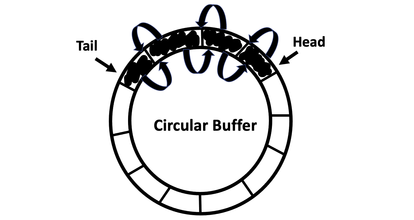
A circular array fixed-size queue has the capability of performing all of the operations described above; but here, I will only describe the functionalities that are necessary for the algorithm:

1) Peek: You can look at the very first element in the queue with a time-complexity of \(O(1)\).

2) Insert: You can insert ('push') an element to the back of the queue with a time-complexity of \(O(1)\). To do this, the underlying algorithm starts by creating a node that contains the new element. It then uses the Tail pointer node to access the last data-storing node in the deque, and changes the pointers of both these nodes to point to the new node. It finally changes the pointers of the new node to point to the previous last node and the Tail pointer node, respectively. Thus, the new node is inserted into the data-structure.

3) Delete: Finally, you can delete ('pop') an element from the front of the doubly linked-list deque with a time complexity of \(O(1)\) by altering the pointers such that the Head pointer points to the node after the 'node to be deleted', so that the node in front of 'the node to be deleted' instead points to the Head pointer.

Implementing the Karplus-Strong algorithm

When a guitar string is plucked, the string vibrates and creates sound. The length of the string determines its fundamental frequency of vibration. So, we first created a guitar string of the specified frequency, using a sampling rate of 44,100. We initialized our circular array fixed-size queue with a fixed capacity of \(n=\)\(44100\over f\), where \(f\) is the frequency of the note being played, rounded up to to the nearest integer, and then enqueued \(n\) zeros to the queue.

We model a guitar string by sampling its displacement (a real number between -\(1\over 2\) and +\( 1\over 2\) at \(n\) equally spaced points in time. The vibrations that result from plucking the string spread wave-like over time. This spreading can be simulated using the Karplus-Strong algorithm. To simulate the initial pluck of the string, all the values in the queue were initialized with white noise from uniformly random values between -0.5 and 0.5. We simulate one time-step of the string vibration by applying the Karplus-Strong algorithm to the queue.

In each step of the Karplus-Strong algorithm, the first sample is deleted from the queue, and a new value is added to the end of the queue - here, the new value is the average of the deleted sample and the new first sample, scaled by an energy decay factor of 0.996. Over multiple time-steps, the Karplus-Strong algorithm simulates a gentle low-pass filter (which attenuates the transmission of higher frequencies while allowing lower frequencies to pass). The figure below illustrates the transition of the queue during a single time-step when acted upon by the Karplus-Strong algorithm.



The Karplus-Strong algorithm essentially approximates a solution of the 1D wave equation, which describes the transverse motion of the string as a function of time. The length of the cyclic queue determines the fundamental frequency of the resulting sound. Sonically, the feedback mechanism reinforces only the fundamental frequency and its harmonics (frequencies at integer multiples of the fundamental). The energy decay factor of 0.996 models the ever-so-slight dissipation in energy as the wave makes a roundtrip through the string.

A more physical interpretation of what's happening here is as follows: when you pluck a guitar string at its center, it sends oscillations of travelling waves on both sides until the tension on the string regulates and dampens these oscillations until they die down. One immediate implication of this is that strings which are tightened to characterize high-frequency notes have a greater tension, which allows them to vibrate faster but also die down faster under its dampening tension. Similarly, low-frequency notes have a lower tension and so vibrate longer since there is no immediate dampening force.

So, when you simulate the string by considering nodes in the cyclic queue as the displacements of the center of the string over time, there are two physical intepretations from the algorithm. Firstly, initializing the queue with white noise from (-0.5 to 0.5) is equivalent to simulating the initial (unpredictable) oscillation of the string with traveling waves on each side from the center. Secondly, averaging adjacent samples from the queue bring them closer to each other, which describes how the string loses energy through the dampening process.

Code Execution

I ran this code through the GuitarHero package: it creates a simulator that supports a total of 37 notes on the chromatic scale from 110 Hz to 880 Hz. The GuitarHero keyboard imitates a piano, such that the white keys are on the asdfghjkl; row and the black keys are on the qwertyuiop[]\ row. However, this software was unfortunately incompatible with HTML, so I found a better alternative:

I used an existing CSS/JS prepackage of a pretty cool piano with 24 keys (with note transitions) but excluded the inbuilt tones from the set-up. I then pre-recorded each note through GuitarHero.



Finally, I wrote a JavaScript command to play these sounds (results from the Karplus-Strong algorithm) upon pressing the corresponding keys. I should comment that I lost 13 additional keys that I generated from the Karplus-Strong algorithm since the pre-existing CSS embedding of the piano only renders 24 keys, but I think it's a pretty good rendition of a piano, so I won't complain about it! This concludes everything I had to say about the construction of of the synthesizer.